> ## Documentation Index
> Fetch the complete documentation index at: https://docs.bioptimus.com/llms.txt
> Use this file to discover all available pages before exploring further.
# Tile embeddings & PCA
> Extract tile embeddings (H-Optimus or M-Optimus) and visualize morphology with PCA.
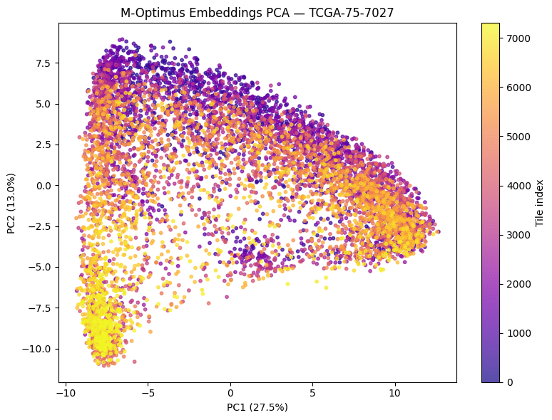
Both H-Optimus and M-Optimus produce a 1536-dimensional embedding per tile (the CLS token). Principal components of these embeddings reveal the dominant axes of morphological variation — often corresponding to tissue vs. background, tumor vs. stroma, and immune-rich vs. immune-poor regions.
`h1-jumpstart` — a full, runnable H-Optimus embedding example.
`m-jumpstart` — the equivalent for M-Optimus.
## 1. Configure the model
Embeddings are available from both models. Import once, then pick your backend and model — the rest of the guide is identical.
```python theme={null}
from bioptimus.models.backbones import Backbone
from bioptimus.models.types import Models
from bioptimus.preprocess.wsi.models.bioptimus_mask import BioptimusTissueMaskModel
from bioptimus.preprocess.wsi.provider.tiled import TiledTissueMask
```
```python H-Optimus theme={null}
API_URL = "http://localhost:8080"
model = Backbone(Models.H1, backend="remote", base_url=API_URL)
tissue = Backbone("tissue-seg", backend="remote", base_url=API_URL)
```
```python M-Optimus theme={null}
API_URL = "http://localhost:8080"
model = Backbone(Models.M_OPTIMUS, backend="remote", base_url=API_URL)
tissue = Backbone("tissue-seg", backend="remote", base_url=API_URL)
```
```python H-Optimus theme={null}
model = Backbone(Models.H1, backend="aws",
endpoint_name="h-optimus", region_name="us-east-1")
tissue = Backbone("tissue-seg", backend="aws",
endpoint_name="h-optimus", region_name="us-east-1")
```
```python M-Optimus theme={null}
model = Backbone(Models.M_OPTIMUS, backend="aws",
endpoint_name="m-optimus", region_name="us-east-1")
tissue = Backbone("tissue-seg", backend="aws",
endpoint_name="m-optimus", region_name="us-east-1")
```
```python theme={null}
mask_provider = TiledTissueMask(model=BioptimusTissueMaskModel(backbone=tissue))
```
## 2. Extract embeddings
```python theme={null}
from bioptimus.inference.inference import SlideInference as Inference
from bioptimus.inference.writers import OutputFormat
inferrer = Inference(wsi_path="/data/wsi/tcga_coad.svs", model=model,
mask_provider=mask_provider, mask_threshold=0.5)
result_path = inferrer.predict(output_path="/data/output/tcga_coad.zarr",
output_format=OutputFormat.ZARR,
max_concurrency=256, mode="embed")
```
On a single-GPU SageMaker endpoint (`ml.g5.xlarge`), lower `max_concurrency` (e.g. 32) to avoid out-of-memory from concurrent tile requests.
## 3. PCA
Load the embeddings and fit PCA in one call — `bioptimus.utils.plot_pca_scatter` fits, plots, and returns the scores plus the fitted PCA (explained-variance ratios are printed):
```python theme={null}
from bioptimus import utils
data = utils.load_zarr_output(result_path)
embeddings, coords = data["outputs"], data["coords"] # (N, 1536), (N, 2)
scores, pca = utils.plot_pca_scatter(embeddings, n_components=3,
title="Embeddings PCA", cmap="plasma")
```
 ## 4. Spatial visualization
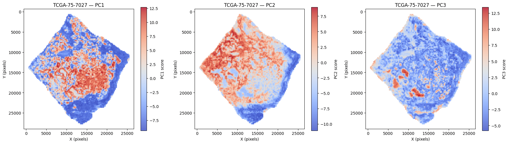
`plot_spatial_pca` maps the PC scores back onto tile coordinates as per-PC spatial heatmaps — each component tends to isolate a distinct tissue compartment:
```python theme={null}
utils.plot_spatial_pca(scores, coords, components=[0, 1, 2])
```
## 4. Spatial visualization
`plot_spatial_pca` maps the PC scores back onto tile coordinates as per-PC spatial heatmaps — each component tends to isolate a distinct tissue compartment:
```python theme={null}
utils.plot_spatial_pca(scores, coords, components=[0, 1, 2])
```
 The same embeddings feed downstream models (classification, clustering, retrieval, MIL). For the high-level workflow with caching and workspaces, use the [Inference pipeline](/guides/get-started/inference-pipeline) with `infer.embed(path)`.