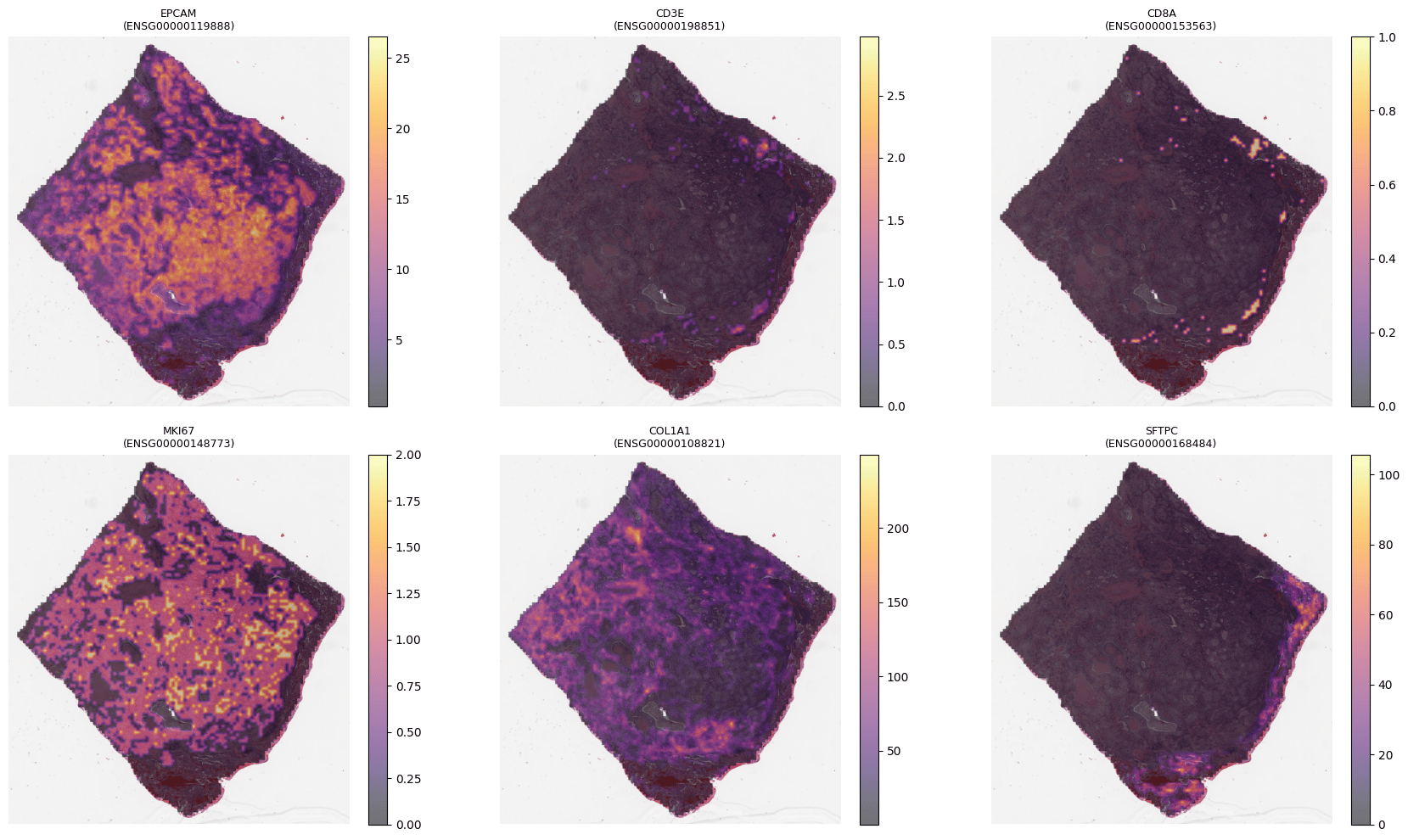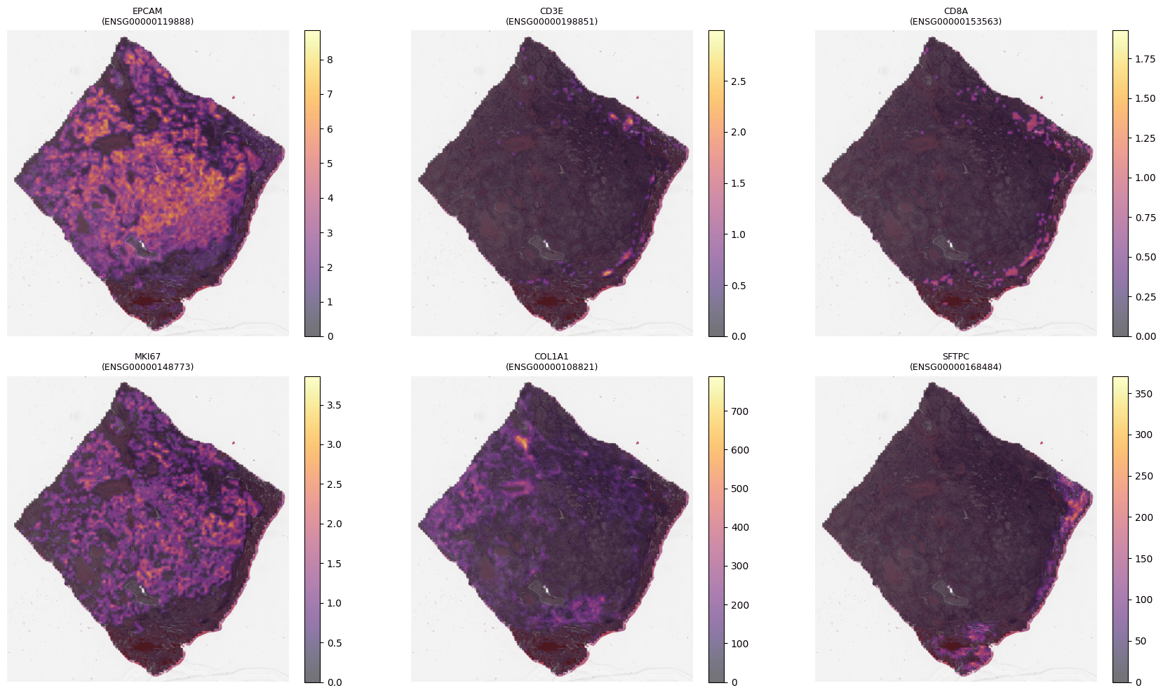

M-Optimus predicts expression of thousands of genes directly from H&E histology — no spatial transcriptomics assay required — enabling spatial analysis on any archived slide. This guide uses the core API (Backbone + SlideInference) for explicit control; the Inference pipeline wraps the same steps.
Runnable notebook
See m-jumpstart for a full, runnable M-Optimus example.
Pick your backend — the rest of the guide is identical for both.
from bioptimus.models.backbones import Backbone
from bioptimus.models.types import Models
from bioptimus.preprocess.wsi.models.bioptimus_mask import BioptimusTissueMaskModel
from bioptimus.preprocess.wsi.provider.tiled import TiledTissueMask
API_URL = "http://localhost:8080"
model = Backbone(Models.M_OPTIMUS, backend="remote", base_url=API_URL)
tissue_backbone = Backbone("tissue-seg", backend="remote", base_url=API_URL)
from bioptimus.models.backbones import Backbone
from bioptimus.models.types import Models
from bioptimus.preprocess.wsi.models.bioptimus_mask import BioptimusTissueMaskModel
from bioptimus.preprocess.wsi.provider.tiled import TiledTissueMask
model = Backbone(Models.M_OPTIMUS, backend="aws",
endpoint_name="m-optimus", region_name="us-east-1")
tissue_backbone = Backbone("tissue-seg", backend="aws",
endpoint_name="m-optimus", region_name="us-east-1")
mask_provider = TiledTissueMask(model=BioptimusTissueMaskModel(backbone=tissue_backbone))
print(f"{len(model.input_gene_names or [])} input genes, "
f"{len(model.output_gene_names or [])} output genes")
2. Run inference (image only)
SlideInference tiles the slide at 0.5 µm/px, dispatches tiles concurrently, and streams results to Zarr so memory stays constant regardless of slide size.
from bioptimus.inference.inference import SlideInference
from bioptimus.inference.writers import OutputFormat
inferrer = SlideInference(
wsi_path="/data/wsi/tcga_coad.svs",
model=model,
mask_provider=mask_provider,
mask_threshold=0.5,
)
result_path = inferrer.predict(
output_path="/data/output/tcga_coad.zarr",
output_format=OutputFormat.ZARR,
max_concurrency=256, # see note for single-GPU SageMaker endpoints
)
Tissue masking filters background tiles before prediction — on a typical TCGA slide this skips most of the ~16k tile grid. Set mask_threshold to the minimum tissue fraction to keep a tile (default 0.5).
On a single-GPU SageMaker endpoint (ml.g5.xlarge), lower max_concurrency (e.g. 32) to avoid out-of-memory from concurrent tile requests. On a multi-GPU on-premise server, 256 is a reasonable default.
3. Add bulk RNA (multimodal prediction)
M-Optimus prediction can be conditioned on bulk RNA for a multimodal readout. Bulk RNA is attached through a Cohort via late-binding: run image-only first, then link the RNA and re-predict. Modality-aware tracking processes only the missing outputs, and image-only results are preserved separately for comparison.
Send TPM-normalized expression values — do not log1p them yourself. The server transforms the input and the model output for you. Genes are auto-aligned to the model’s input set; genes the model expects but your file lacks are encoded as -1 (non-measured).
The server applies two transforms around the model:
| Stage | Transform | Applied to |
|---|
| Input (preprocess) | log1p | your TPM-normalized expression values, before the model |
| Output (postprocess) | expm1 | the model output, to return expression values |
from bioptimus.data.cohort import Cohort
from bioptimus.inference import Inference
from bioptimus.models.types import Models
cohort = Cohort.from_directories(wsi_dir="/data/wsi/tcga_mini_coad")
infer_m = Inference(model_name=Models.M_OPTIMUS, cohort=cohort,
api_url="http://localhost:8080", tissue=True,
output_path="/data/output", experiment="tcga_coad", run=1)
infer_m.run(mode="predict") # image-only baseline
Link bulk RNA and re-predict:
# Plain CSV (Ensembl IDs as columns):
cohort.link_bulk_rna("/data/rna/tcga_mini_coad")
# GDC/TCGA gene-quantification TSVs — use the tpm_unstranded column (not
# fpkm_* or raw counts) and strip Ensembl versions:
cohort.link_bulk_rna(
"/data/rna/tcga_mini_coad",
gene_column="gene_id",
value_column="tpm_unstranded", # TPM-normalized expression values (the expected scale)
strip_version=True, # ENSG00000000003.15 -> ENSG00000000003
)
infer_m.run(mode="predict", force=True) # re-predict with bulk RNA context
Retrieve each stage’s output by modality:
out = cohort[0].outputs.get(infer_m.model_name)
img_only = out.get_stage_path("predict", ["image"])
multimodal = out.get_stage_path("predict", ["image", "bulk_rna"])
4. Inspect the output
Load either output — image-only or multimodal — with the built-in helper:
from bioptimus import utils
data = utils.load_zarr_output(result_path)
outputs, coords = data["outputs"], data["coords"] # (n_tiles, n_genes), (n_tiles, 2)
gene_names = data["gene_names"]
5. Visualize
Genes are identified by Ensembl gene ID (e.g. ENSG00000198851). Useful markers include EPCAM (ENSG00000119888, epithelium), CD3E (ENSG00000198851, T-cells), CD8A (ENSG00000153563, cytotoxic T-cells), MKI67 (ENSG00000148773, proliferation), COL1A1 (ENSG00000108821, stroma), and SFTPC (ENSG00000168484, alveolar).
bioptimus.utils.plot_gene_panel_overlay renders a whole panel on the slide thumbnail in one call. Load the two prediction sets from step 3 and compare them — the multimodal output uses bulk RNA, the image-only output does not:
from bioptimus import utils
GENE_PANEL = {
"EPCAM": "ENSG00000119888", # epithelium / tumor
"CD3E": "ENSG00000198851", # T-cells
"CD8A": "ENSG00000153563", # cytotoxic T-cells
"MKI67": "ENSG00000148773", # proliferation
"COL1A1": "ENSG00000108821", # stroma
"SFTPC": "ENSG00000168484", # alveolar (lung)
}
bulk = utils.load_zarr_output(multimodal)
utils.plot_gene_panel_overlay(bulk["outputs"], bulk["coords"], bulk["gene_names"],
GENE_PANEL, wsi_path=wsi_path, cols=3, cmap="inferno")
image = utils.load_zarr_output(img_only)
utils.plot_gene_panel_overlay(image["outputs"], image["coords"], image["gene_names"],
GENE_PANEL, wsi_path=wsi_path, cols=3, cmap="inferno")
A FP16 model variant is available for faster inference. Run the FP32 and FP16 outputs through the same analysis to compare the impact of quantization.